Wall Street University: Betting Markets (Part IV)

 It’s been a long road, but this chapter and the next discuss the main topics we've been building to.

Part IV discusses:

• The Optimal Bets
• Combining bets into mini (2 asset) portfolios
• Conditional values and hedging

Part V is the complete and generalized version of these topics.  Part V extends the investment process from 2 assets to all 260 assets and uses Portfolio Theory to find the optimal combination of investments.

This Series

Part I: The Power of Models

Part II: Building Blocks & Covariance

Part III: PredictIt & The Mechanics of Markets

Part IV: The Best Bets (Statistically) & Two-Bet Portfolios

Part V: Optimal Portfolios & The Efficient Frontier

Part VI: Polling Models, Internal Models & Large Portfolios > $20,000

Part VII: The Math, The Code & Visualizing 10,000-Dimensional Spaces

Part VIII: 2018 Elections & Becoming a Portfolio Manager

‘Yes’ vs. ‘No’

I mentioned previously that PredictIt has 130 markets for the presidential election. However, the investment model uses 260 assets.

The reason for this doubling, is that ‘Yes’ bets and ‘No’ bets have to be treated as different objects, rather than simply ‘Long’ and ‘Short’ positions in that market.

Why?

Fees, Risk-Free Rate and Leverage

There are three reasons why a market cannot be treated a single asset to long or short.

The first reason is the fee structure. The 10% fee on profits, but no fee on losses, makes the problem nonlinear. This means that we can't think of it as just being a positive or negative of the same value.

Second, there is the concept of Risk-Free Rate. Every economy and currency has a basic cost of money, the return an investor can expect with certainty that their capital will be returned to them (risk-free). In most economies this is considered to be the savings rate at a bank or a safe government bond. In the US this is about 0–2%, depending on the duration.

For investments, the risk-free rate is the benchmark minimum against which a risky asset must exceed. If it doesn't pay more than a riskless bond, then why gamble?

In the PredictIt ecosystem, I would argue this rate is approximately 10%.

There are always markets on PredictIt which offer a return of 8-10% with perhaps 1% chance of loss. There may not be a “PredictIt Bank” that pays 10%, but if capital on the site could be invested in one of these markets, it would never make sense to enter a risky bet (like presidential markets) unless the Expected Return was greater than 10%.

That is the prerequisite to relevance.

The third reason is leverage. If a market is at 80, a seller can get 4x the leverage for the same $100 invested (500 shares vs 125 shares).

$1 vs. 1 Share

Let's talk about units for a moment.

When setting up the Portfolio Management model, there are two ways to set the units. One is to make the fundamental unit = 1 Share (e.g. Buy Yes at $0.80 or Buy No at $0.20). The other method is to set the unit = $1 invested in each asset.

For reasons that I’ll explore fully in Part VII, the problem is cleaner to set up and understand if all 260 assets are treated as $1 invested.

This system of units also makes the $850 limit a bit easier to manage mathematically.

260 Vectors

We ended the last chapter where the output from the Monte Carlo was a 10,000 x 130  array of 0’s and 1’s.

Essentially for each of the 130 markets, the model made a vector of 10,000 possible outcomes, each a 0 or 1.

I’ll call those the ‘Market Vectors’.

Now we transform the market vectors into ‘Portfolio Vectors’.

For each market, 2 portfolio assets are created (Yes and No). The Yes Vector is the profit from $1 invested as Buy Yes in the market. The No Vector is the profit from $1 on Buy No.

These vectors include all the effects of fees and the assumption of 10% risk-free rate.

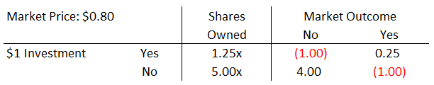
To incorporate the risk-free rate, I will treat it as a Cost of Capital or Opportunity Cost and subtract 10% of the market price from the payouts.

Therefore, if a bet is lost, the total cost will be $1.10. This equivalent to losing $1 which could have been invested in an ‘easy money’ bet instead, yielding $1.10.

If a bet is won, the net profit will be the returns, minus fees (10% of profit), minus the cost of capital (10% of the market price).

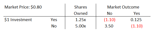
Here, winning a Yes bet means buying at $0.80 and settling at $1.00.  Fees are 10% of $0.20 profit, or $0.02 (per share).  The cost of capital is 10% of the $0.80 cost (per share).  For a total of $0.20 - 0.02 - 0.08 = $0.10 per share.

Since $1 would buy 1.25 shares at $0.80, the total profit is 1.25 x $0.10 = $0.125.

The same calculations for No would involve buying 5 shares at $0.20.

Check that you get the same values as the table above.

Finally, with all of the fees and complexities baked into the net profit numbers, we can now produce the 10,000 x 260 Portfolio Vectors.

This output represents how 130 markets both Yes and No (130 x 2 = 260 ways to bet) across the 10,000 simulations, each in terms of $1 wagered.

If this isn't totally clear, I suggest re-reading this section one more time.

Optimal Bets

It’s been a long journey and we are 12,000 words into this series. Now, the part I (perhaps) should have led with.

Drum roll please…

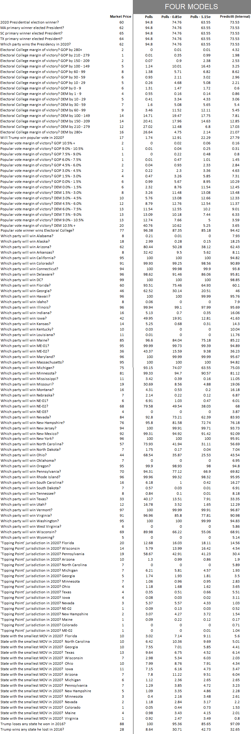
Here is a table of all the markets and the expected value from each of the four models.

Unless otherwise stated, all Presidential and State markets are priced from the point-of-view of Biden winning.

For example Pennsylvania at 70, means the market prices a 70% chance of Biden winning or a 30% chance of Trump.

Expected Value

As promised, let’s focus on the Polls - 0.85σ Model.

What is the expected return for each of the 260 markets?  Which bets are worth taking and which are not.

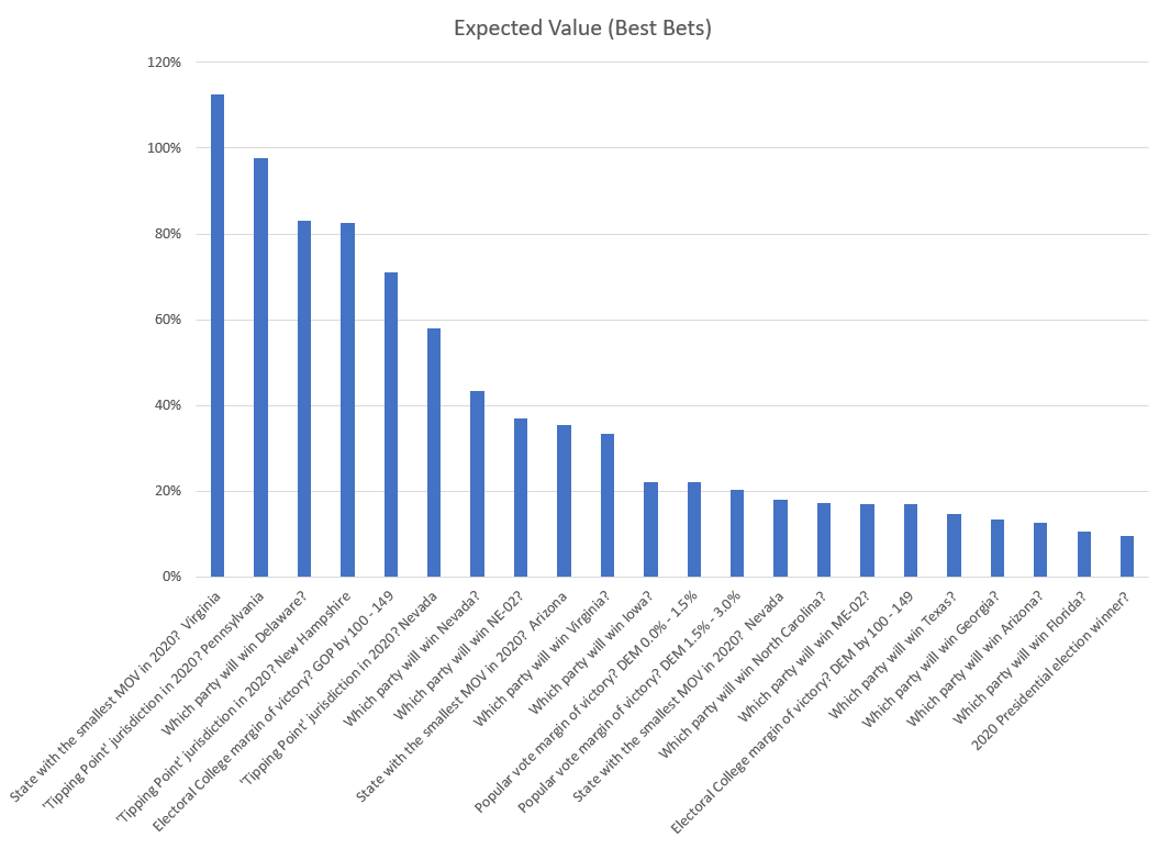
Below is a bar chart of all 260 markets in terms of a $1 bet.

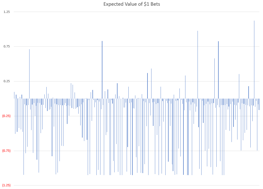
Only a few bets have an expectation of profit.

Like most markets, the majority of investments are barely better than chance. You can see from all the negative values that most bets are a net loss after accounting for fees and interest.

But unlike many other investment markets, 15% of the PredictIt bets seem to be winners, —  and half of those offer serious opportunities.

Let’s narrow our focus to the 22 bets that offer a positive expected value, greater than 10%. (That’s 10% after the 10% cost of capital already taken out, so actually 21% profit).

These are most profitable opportunities.  If we were to stop here, you would have a good palette of wagers.

Next we will examine these more closely, consider various risks and learn how to combine different bets into a guaranteed profit.

Observations

Before we move on, a few notable patterns jump out in these 22 assets.

Biden vs. Trump

Many of the bets fall along clear partisan lines. A given state will be won by Biden or by Trump.

The presidential race is the purest form the partisan bet. Other bets are a sub-set of this binary event — for example, “Electoral College GOP to win by 100–149” which can only win in the subset of cases where Trump wins.

But not all bets have a partisan component...

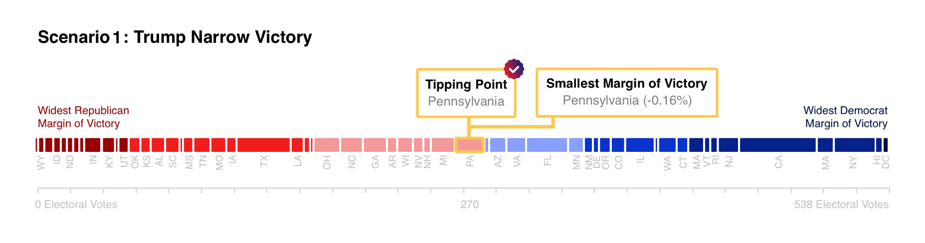
Take for example the bets on Tipping Point states. Tipping point bet is about the median state on the political spectrum. If all of the 56 jurisdictions are ranked by the margin of their vote and we started counting from the most Republican (or most Democratic), adding the electoral votes as we go along, which state would give the 270th vote? That is the tipping point.

Full rules for Tipping Point

This market is more a bet on current polling and a large degree of randomness/statistics. Which states wins this market has very little to do with the overall winner.  This is also probably the most interesting bet for our model.

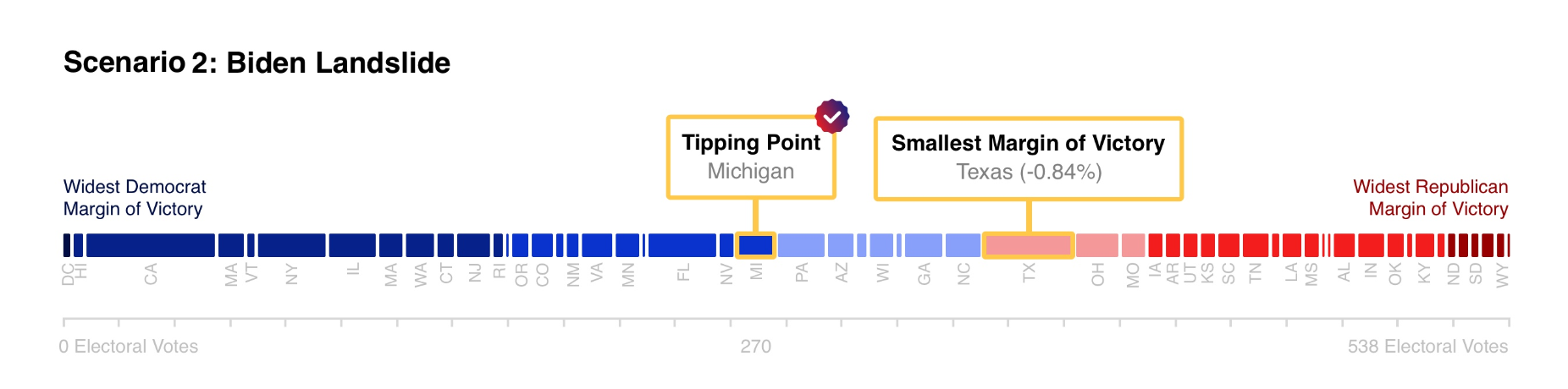
Smallest Margin of Vote however is very partisan. This is just a backdoor way of voting on the Electoral Margin.

As an example,  here is a simulation where Texas has the smallest margin of vote (closest race).  Since Texas is typically a safe bet for Republicans, this implies that Biden has won the majority of the map.

Bid/Offer

The next observation to consider about these markets is that I’ve treated the market price as a single number. In reality if you want to Buy Yes or Buy No, you will pay a slightly different price (the bid/offer spread).

For most of these markets the impact of $0.01 of spread is negligible, but for markets with very low (or very high) prices, the $0.01 consideration becomes large.

Take for example, the best bet from the bar graph: Virginia as smallest Margin-of-Vote (MOV).

Virginia has a market price of 1. But in reality, the bid/offer is actually 1 / 2 (pronounced “one at two”), meaning that lowest price someone is willing to sell right now is $0.02 and the highest someone is willing to pay is $0.01.

As a buyer, you have two options, either pay 2 right now (which is not an attractive investment) or place a limit order to buy at 1 and “Get Filled” (your order is executed because a seller traded at your limit price).

Note: Since it's onerous to always write in $ and decimals, I typically use the format of whole numbers and neglect the $ sign.

Conversely, the second-best bet is Pennsylvania as the tipping point jurisdiction. This market is trading at 19. The actual market is 19/20 and the model has the expected value as 41.

Here the bid/offer is more negligible.

Even after fees, opportunity cost and $0.01 of bid/offer spread, this market offers about 100% expected return if you buy at 20 for something that is worth 41.

Certainly not a sure thing but, worth the risk.  

That is to say that 60% of the time you’ll still lose your investment and 40% of the time you’ll get 5x returned.

In later parts of the series, I address how to incorporated this bid/offer effect to show the value for market orders (instead of limit orders).

Negative Correlation

It should be noted that — although these 22 bets are the most profitable in isolation, they aren’t the only markets that matter.

Some combinations of 2 or 3 bets (portfolios) are better than any 1 bet on its own. When I say Better, technically I’m referring to improving the Risk vs. Reward characteristics.

A portfolio is superior to another portfolio if it offers more profit for the same risk, or less risk for the same profit. (More on this in the Pareto Efficient section below).

And unlike in real markets, with PredictIt, we have reliable inputs to our portfolio construction.

Because of the Diversification effects, many of the other 238 bets not listed here are still components of an Optimal Portfolio and part of a balanced breakfast.

If two bets with negative correlation are combined, much of the overall variance is muted, but the profit is additive. More profit, less risk.

Winning Every Time

There are many risks and binary events that could occur in the election, but by far, the largest confounding variable is the overall outcome of the election (Biden vs. Trump).

The concept of the big risks that affect all bets versus small and local risks that affect only some investments is known as Systematic vs. Idiosyncratic risk.

First we will focus on limiting Systemic Risk.

Conditional Probability

Up to this point, we’ve focused on the global expected value. That is the weighted probability of how much profit a $1 investment would yield across all 10,000 simulations.

There has been no consideration for how these bets would fare in the limited case of just Biden winning, or just Trump winning.

Let’s introduce the concept of Conditional Probability, or conditional expected value. That is, what would you expect your profit to be on the condition that I told you Biden won, but given no other information?

You could easily calculate this value by narrowing your calculation from all 10,000 simulations down to the 7,476 where Biden wins, then taking the average.

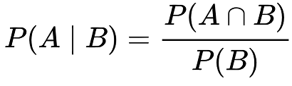
To put it more specifically, the probability of Event A occurring, given that Event B occurred is equal to Both Events occurring, divided by the probability of Event B occurring.

Using a win in Ohio as an example:

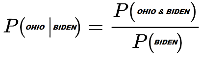
The way to read the left side of the equation is "Probability of Ohio conditional on Biden" or "Probability of an Ohio win given an overall win".  'Conditional on' and 'Given' are often used interchangeably.

Joe Biden has a 35.9% chance of winning Ohio overall.

But in the cases where Biden wins the presidency, he has a 47.2% of winning Ohio. That is he wins both Ohio and the White House in 3,531 simulations and wins the White House in 7,476 in total.

Therefore 3,541 / 7,476 = 0.472 conditional probability of winning Ohio.

Similar work can be done to show Biden wins Ohio and loses the Presidency in 46 simulations (0.46% probability).

Conditional Expected Value

The same method can be extended to calculate the conditional expected value for each bet.

Here’s a table of 6 bets with positive expected value. Notice how the conditional values disperse by Biden vs. Trump:

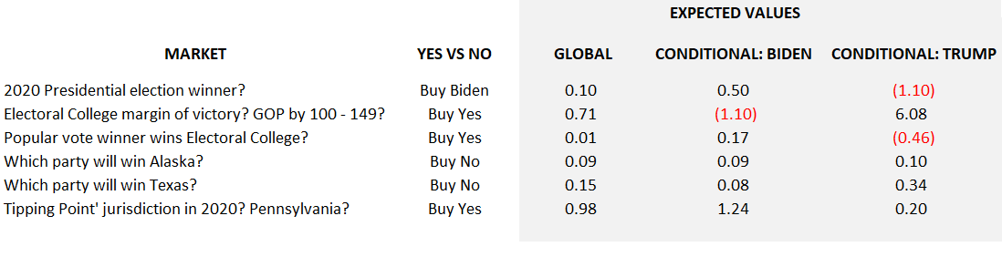
The first market, Presidential Winner, is a pretty obvious example. When Biden wins a bet on Biden pays your $1 plus $0.50 (after fees and 10% cost of capital). The same bet loses if Trump is the winner.

The second example is more interesting. Of course if Biden wins, its impossible for the GOP to win by 100–149 electoral votes (unless Joe and Donny swap parties in October). But conditional on the GOP winning the electoral college, the expected value of a bet on the +100–149 bucket is 6-to-1!

Perhaps combining bet 1 and bet 2 would be preferable to either bet alone? (That’s correct)

Other markets like Alaska, Texas and tipping point Pennsylvania are winning bets in either case. They may have a general slope toward one candidate, but the expected return is positive in either case.

This is not to say that those bets are riskless! Far from it.

It is just a statement that they are generally robust to the systematic risk (Biden vs. Trump). Within those outcomes, any of these bets can still lose in specific simulations. Remember Biden winning is still 7,476 unique scenarios. Trump winning is 2,524 different states as well.

Winning Combinations

Clearly, there are some bets that are desirable in both outcomes and even more two-bet combinations that meet this criteria.

This is where I started plotting the conditional returns on an X, Y axis for easy visualization.

A quick scatter plot of all 260 assets shows that most are phenomenally poor bets.

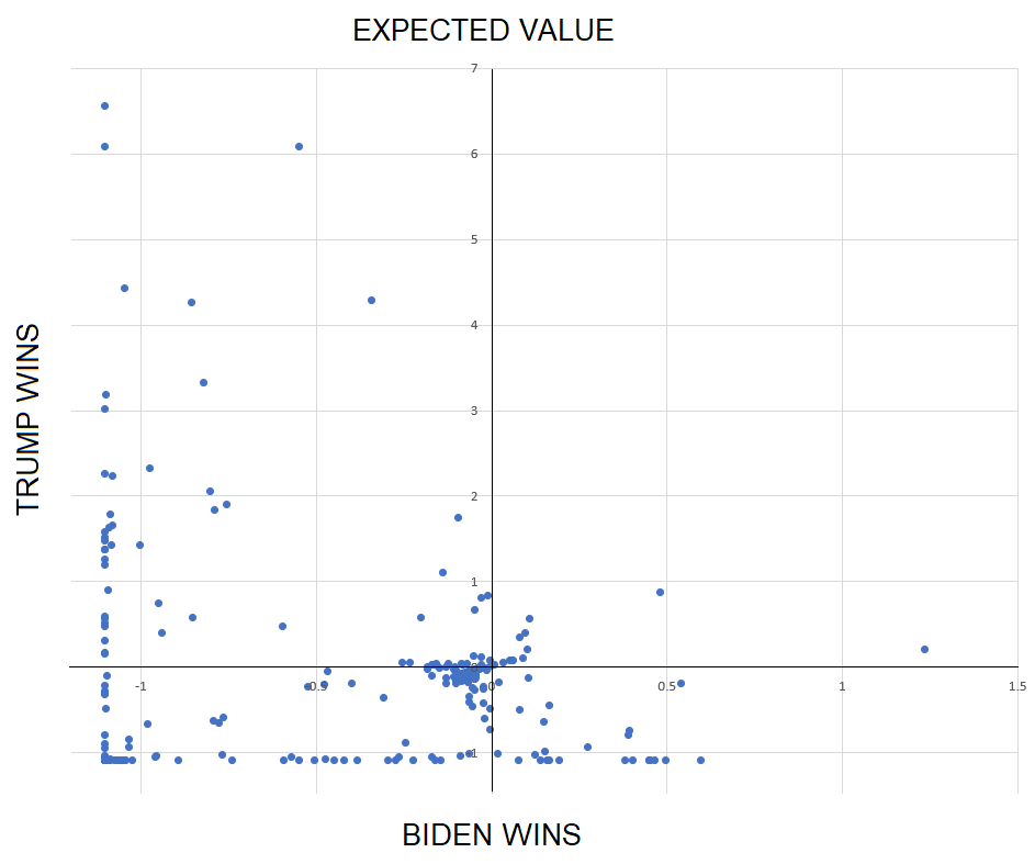
Most of the bets are actually a bad investment whether Trump wins or Biden. This is the lower-left quadrant of the graph.

Efficient Frontier

Let’s focus on the minority of wagers which are positive (or nearly positive) for both outcomes. (Zooming in to the upper right of the last graph.)

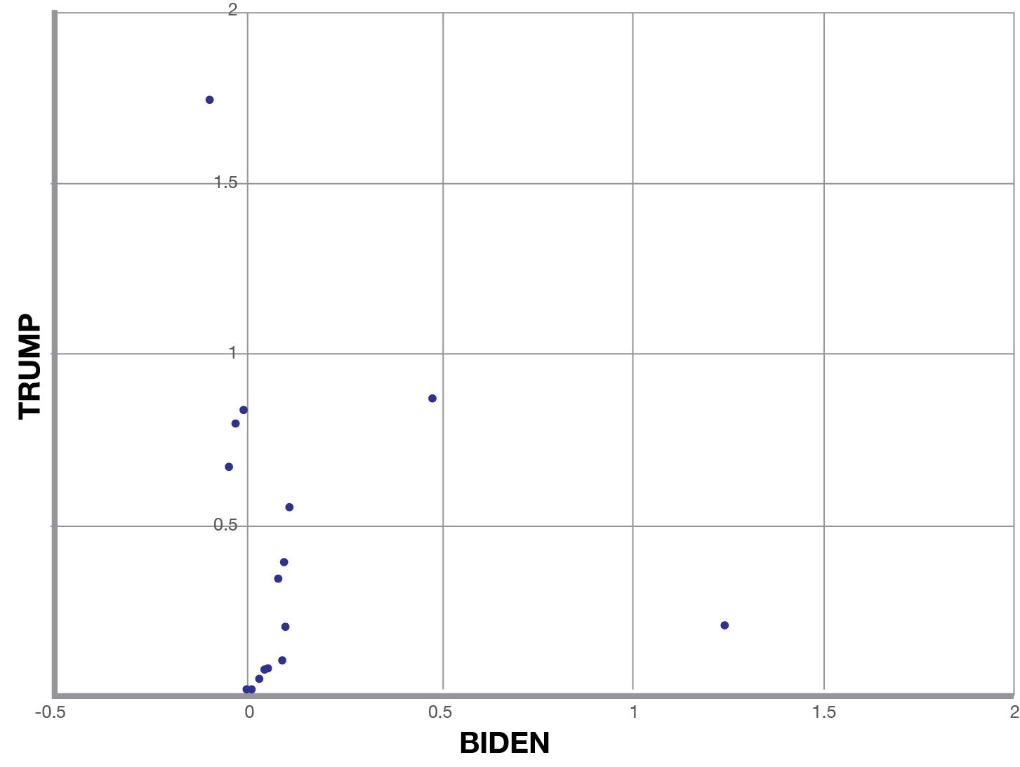
Only 13 assets meet this the positive-positive criteria on their own (one-asset portfolio). The scatter plot includes some other assets which are only mildly negative for one candidate but strongly positive for the other.

Staying for a moment with idea of one-asset bets, which wager is the best?

Depending how you phrase that question the answer can vary. Generally speaking there is an Efficient Frontier of bets which are relatively optimal.

One-to-One

One good heuristic for comparing options would be to accept a trade-off of $1 of opportunity in one candidate for $1 in another candidate.

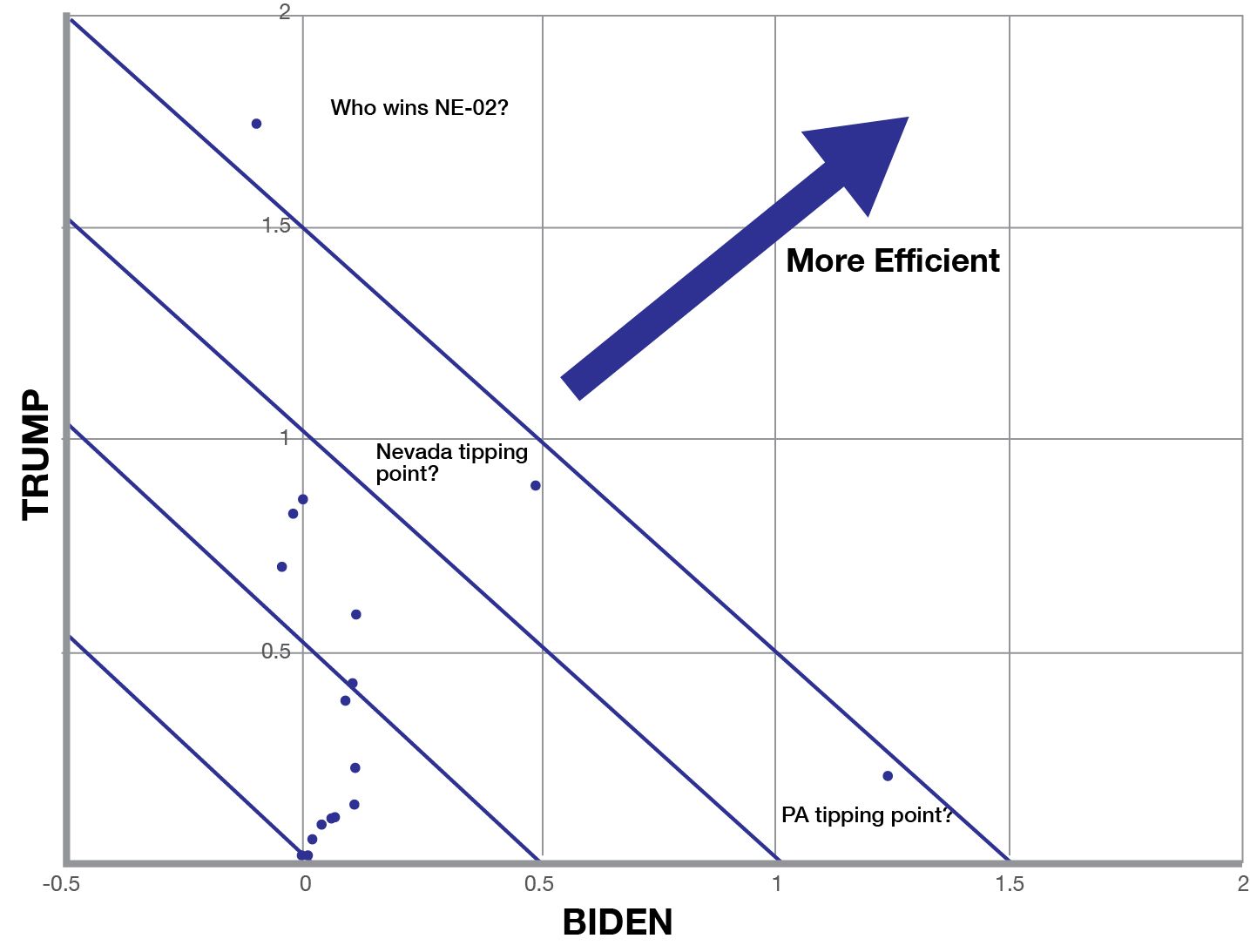
The blue lines are indifference edges. Any point along one of these line would be equal in opportunity to any other point along the same line since you would be trading opportunity in one dimension for an equal value in the other (one-to-one).

I added several parallel blue lines to show higher and higher values of opportunity (efficiency).  The more upper-right a market places, the better the opportunity.

Here, betting on Trump to win Nebraska’s 2nd congressional district (NE-02) appears to be the best option.

Note that this bet does not have a positive expected value in both axes. But the value in the Trump scenario is positive enough to overcome a small negative value in Biden and still have the best net characteristics.

Nevada tipping point and Pennsylvania tipping point also earn an honorable mention.

Pareto Efficient

Another famous heuristic is Pareto Efficient or “Pareto Optimal”. This is method is more restrictive.

Generally speaking, one action is Pareto optimal to another if it is better in any way, without diminishing any other quality.

Given a choice between a trip to Paris, a trip to Rome, and a trip to Paris with free coffee, it’s clear that the third option is Pareto optimal to the first. But this method makes no statement about the relative ranking of the second and third option (croissant vs. cannoli).

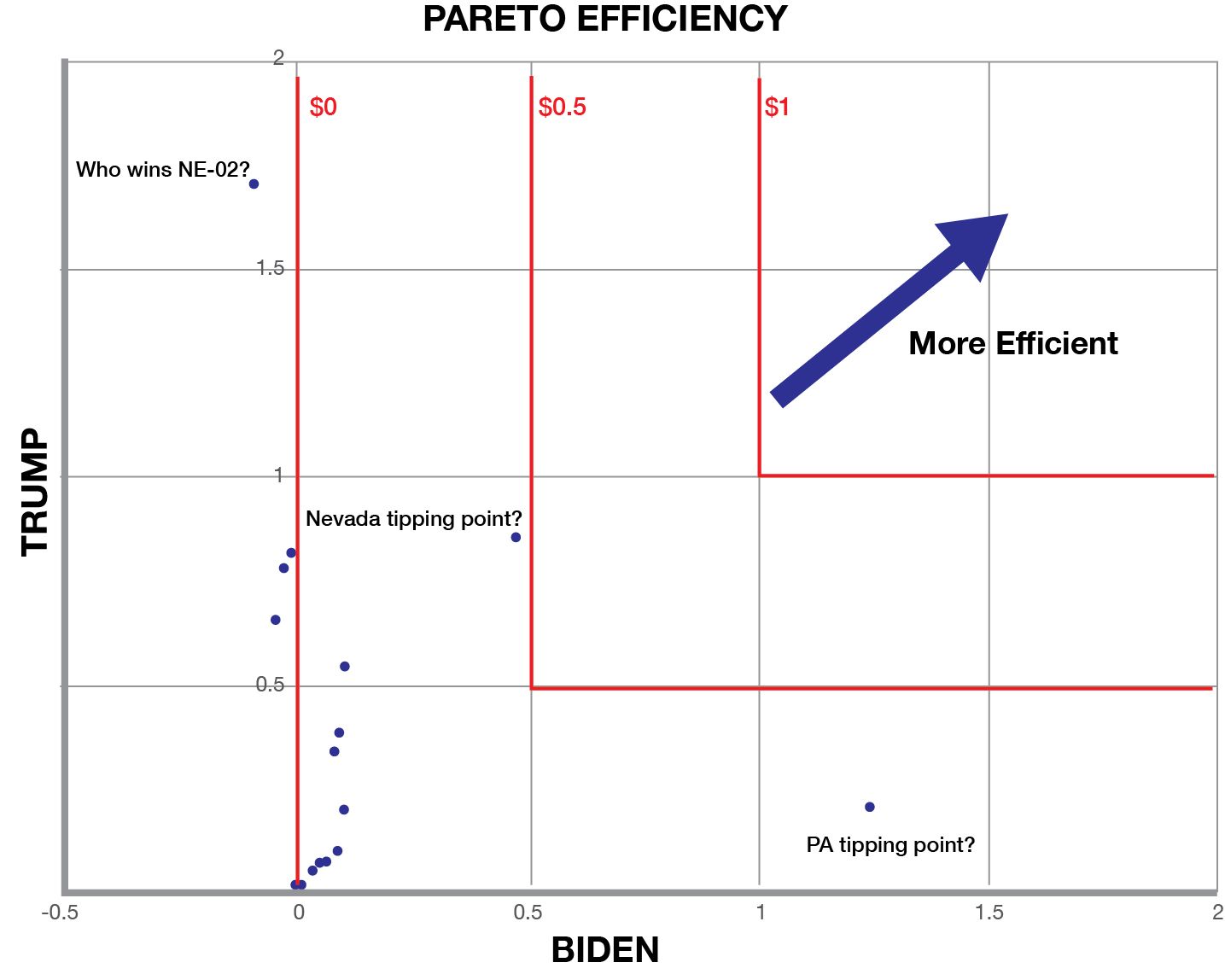
For this XY scatter, this is equivalent to saying an asset is as strong as it’s weakest quality.  Here the Red lines are the indifference edge in the Pareto method of comparing options.

By this metric, Nevada tipping point is the best bet followed by Pennsylvania. But Nebraska-02 is now among the least desirable investments.

When comparing the Pareto and One-to-One, its important to remember that there is no one-size-fits-all approach.  Both have their merits.  Pareto is more conservative, one-to-one is more profit-seeking, both are valid.

In Part V, both of these heuristics will take on a more mathematical definition as we generalize into Portfolio Theory.

Two-Asset Portfolios

Advancing to two-asset portfolios, I mapped out all 33,930 possible combinations of the 260 assets into groups of two-assets.

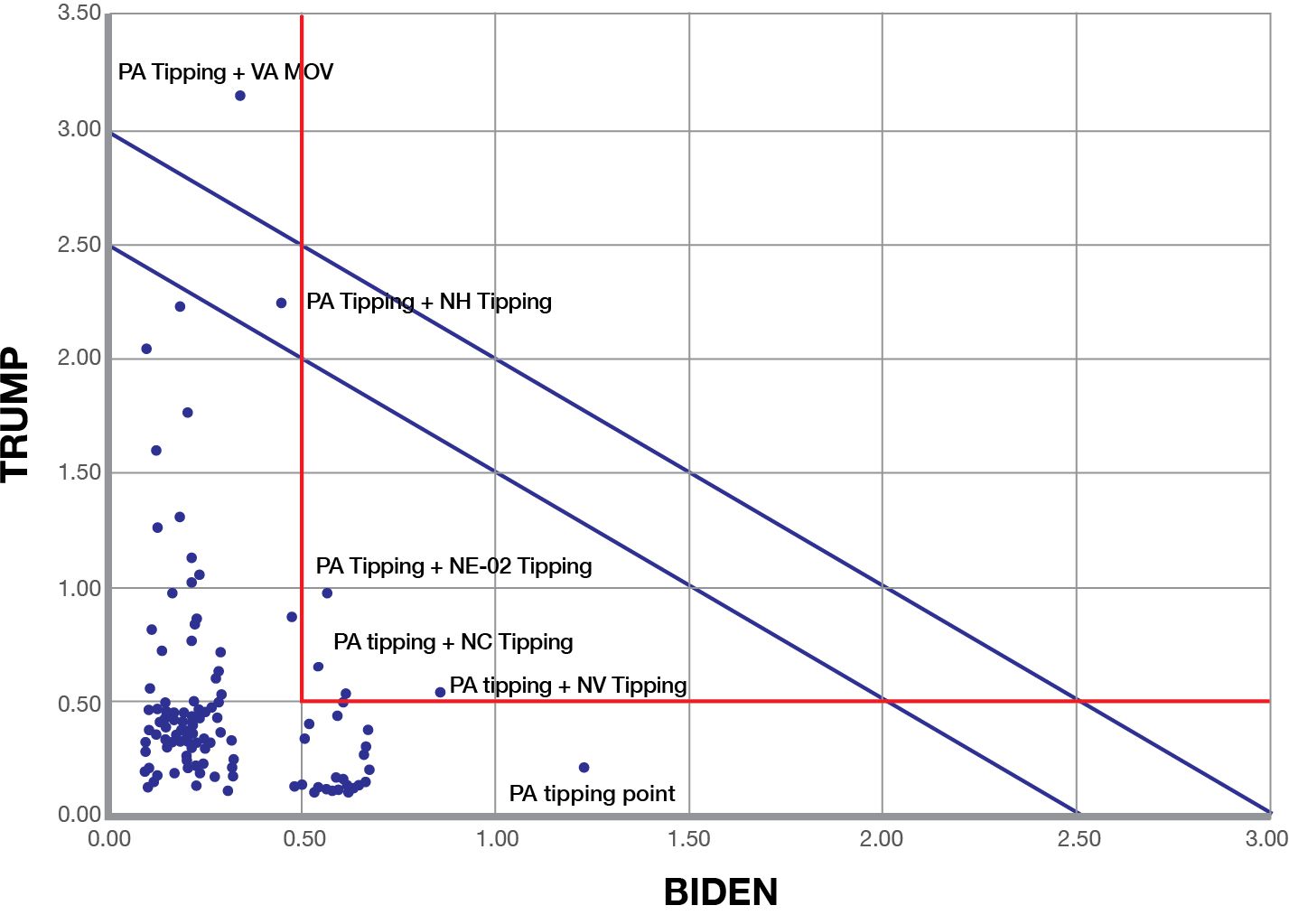
Again most of the combinations were a terrible investment. Let's focus on the minority which are win-win.

Here is a scatter of the best 392 mini-portfolios. This represents the best 1.15% of solutions to the two-asset problem, specifically the options with an expected value over 10% in both axes!

The scatter shows the upper-rightmost Pareto and One-to-One frontiers.

Pennsylvania Tipping Point is in all 6 of the best portfolios.

Three Asset

If we were to proceed in this mechanical method, it next makes sense to try three asset portfolios, or different weights between the assets other than 50/50, or we could focus on the best 10–15 options in the upper right and average them all.

Further, this method is only considering the systematic risk of Biden vs. Trump. It does not hedge the idiosyncratic risks.

The Pennsylvania Tipping Point bet looks pretty sexy, but it’s no Chuck Norris. Even this wager is only projected to win in 43% of cases.

The aim is for a portfolio that wins every time, or as close to 100% as possible and maximizes profit.

To find the best options in this 261-dimensional space (260 independent weights and 1 objective function), we will need a more mathematical approach.

Part V: Optimal Portfolios & The Efficient Frontier (Due to be published next week) introduces Portfolio Theory and other methods to maximize utility.

Collaboration

For any interesting projects or research, or if you just want to discuss some topic, please reach me at: nickyoder10@gmail.com

Don't forget to sign up for weekly updates to the model, polls and optimal Bets!  As market prices change, public polls change and the time until election decreases, I'll update these every week.