The Kelly Criterion

Most traders have heard of the “Kelly Criterion”.

Developed in 1956 by Bell Labs scientist John Kelly, the formula applied the newly created field of Information Theory to gambling and investment. The formula calculates the proportion of one’s net worth to wager in order to maximize the expected logarithm of wealth increase (i.e. geometric growth rate).

Although the Kelly Criterion is commonly mentioned in betting and financial circles, it is poorly understood. Its misuse has led to the ruin of many would-be practitioners.

This two-part series will give a framework for thinking about risk and sizing.

• Part I: Simple mental models and a single-asset application of the Kelly criterion.
• Part II: Multiple assets, correlation and extreme tail risk.

The two cardinal problems in investing, trading or professional gambling are:

1. Finding a set of profitable opportunities
2. Sizing your investments/bets

Most professional traders agree that the second problem is the more difficult of the two.

Instances of this problem include a blackjack player deciding what percentage of his bankroll to wager on a given hand, a real estate investor deciding how much of her portfolio to commit to a new property, and a derivatives trader deciding what leverage to apply to a new strategy.

For many investors, finding opportunities is easy relative to the problems of position sizing and risk management.

“Trading correctly is 90% money and portfolio management.” -Michael W. Covel-

Put another way: A trader with mediocre strategy and a great risk model will become fairly successful. A trader with a great strategy and a mediocre risk model will become bankrupt.

A Simple Example

Imagine a betting opportunity which offers positive expected value with known payouts and probabilities. For example, a card counter playing blackjack who knows that the current Running count and True count imply a win/loss probability for the next hand of 52% vs 48%.

(In the interest of simplicity we will ignore minimum bets, blackjacks, pushes, insurance and the various other edge cases.)

A 52% chance of winning is certainly attractive, but how much of the gambler’s total bankroll (net worth) should he wager on the next hand?

He must balance the competing forces of betting more to achieve greater profit and betting less to limit the chance of going bankrupt.

Somewhere between the extremes, there should be an optimal proportion of total bankroll to bet, such that long-term wealth is maximized.

We can experiment empirically with different bet sizes to see how net worth changes over time. Let’s begin by assuming that the gambler wagers 1% of his net worth on each hand. Here’s a chart of his net worth over the course of 1,000 simulated hands:

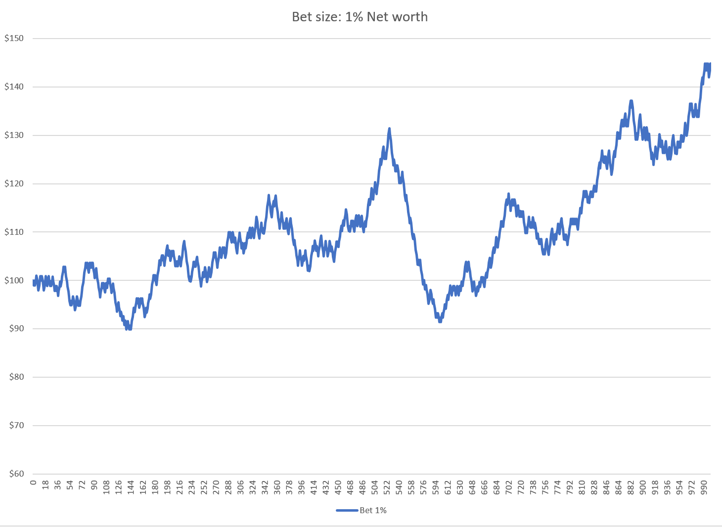
This strategy makes a nice return over time, with a bit of volatility. After 1,000 hands, the gambler has increased his wealth by 44%.

What if the gambler risks a larger proportion of his net worth on each bet? The next chart shows his profit over time with bet sizes of 1%, 2%, and 4% of net worth per hand:

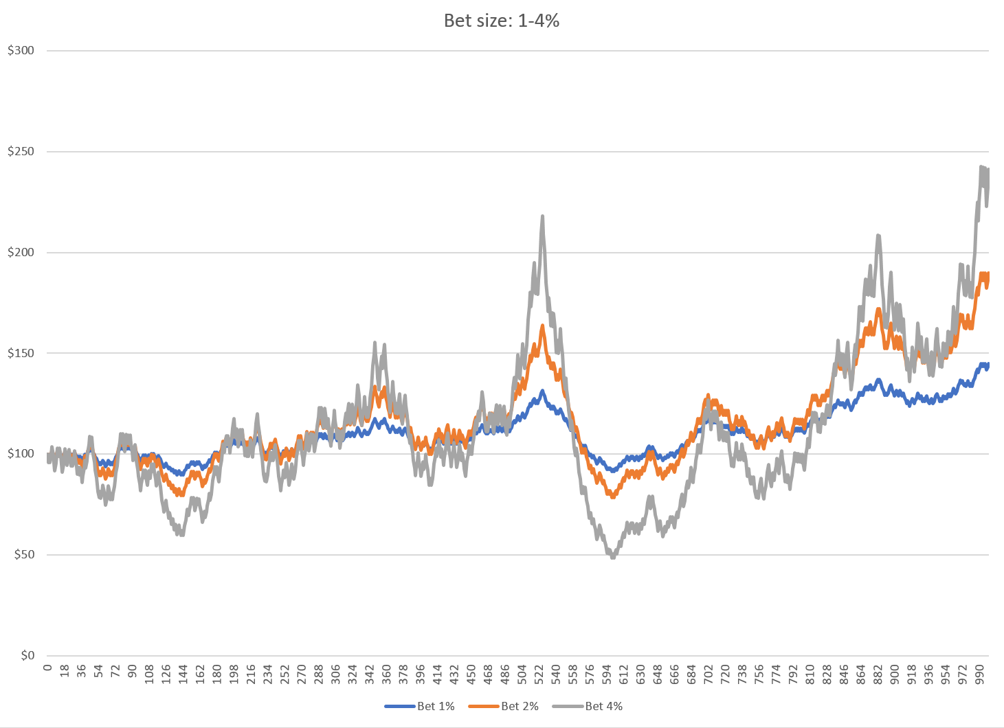
It’s not surprising that as the bet size increases, so does the profit and the variability of our gambler’s net worth.

We can continue testing even larger bet sizes:

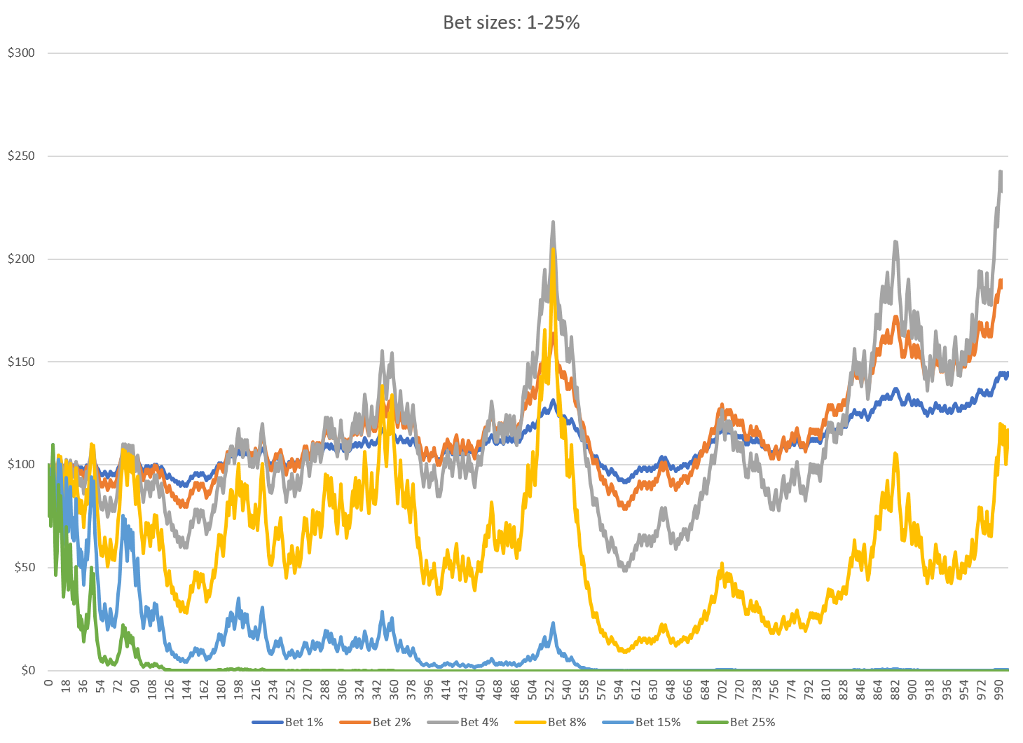
Now something counter-intuitive creeps into our simulation. While our cumulative winnings steadily increased as we increased our bet size from 1% to 4%, we see that 8% does markedly worse and 15% and 25% take his net worth to ZERO (essentially).

The variance of his net worth continues to grow, but his profit reaches a peak and reverses. The wealth-destroying effects of big bets are easier to see with a logarithmic scale.

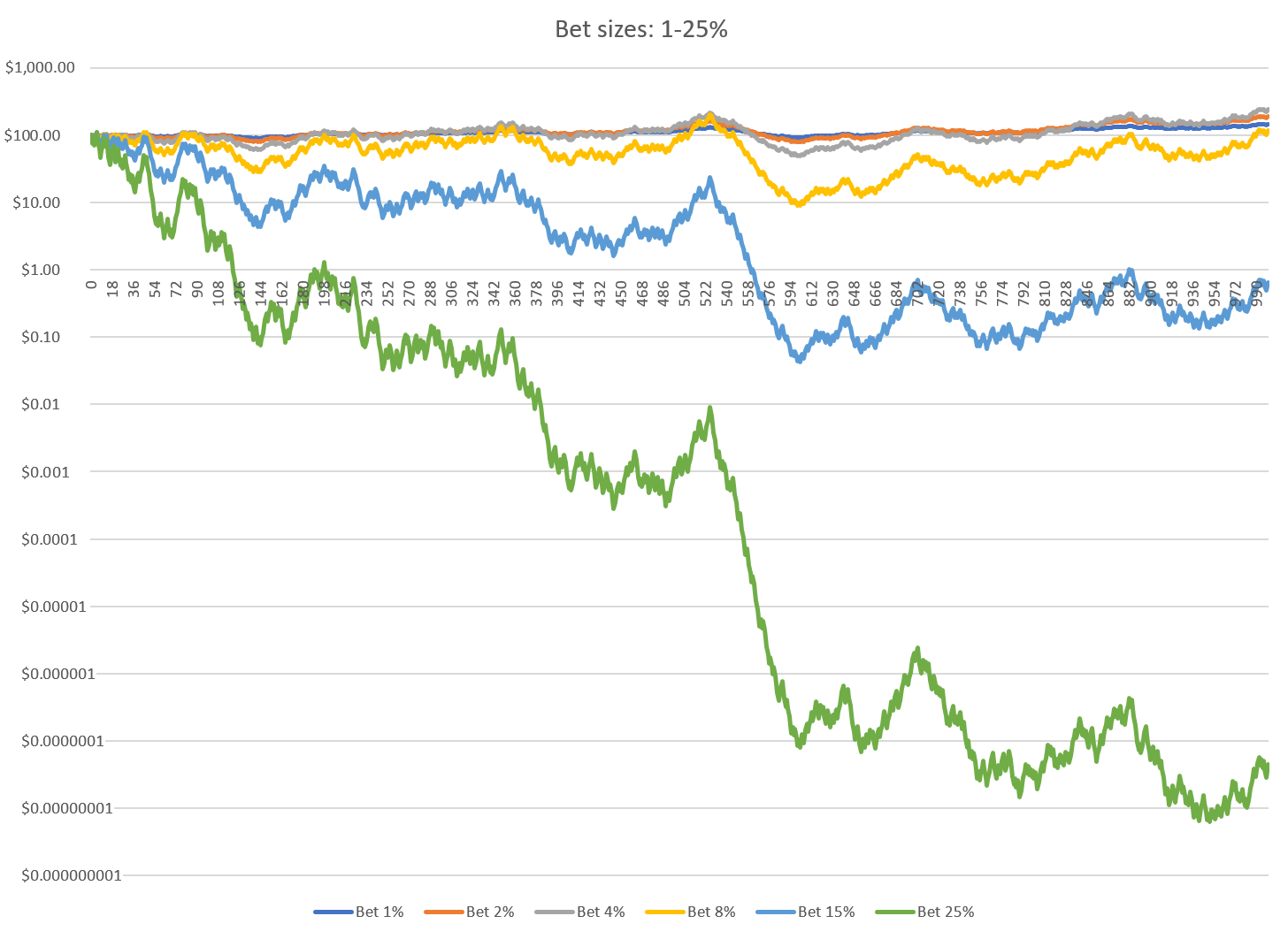
The results of this simulation raise a broader question: given a profitable opportunity, why would doing more of a good thing result in a worse long-term outcome?

The Numbers

Let’s explore with a new example: You’ve found a unique investment. There’s a 50/50 chance of gain or loss, with a gain of 6% and a loss of only 5%. You can choose to make your bet as large or small as you like (i.e. use leverage) up to the possibility of total loss.

Previously we used 1,000 successive bets as a proxy for long-term wealth creation. Now we will simplify the example to two successive bets, one win and one loss. In the long run, the proportion of wins/losses experienced will approach the average win/loss rate of 50/50. Furthermore, because we are looking at the compound growth of our investment, the order of outcomes doesn’t matter. Thus considering two bets with opposing outcomes provides a reasonable estimate of the Geometric Growth Rate of the investment.

A table of profit after one win (+6%) and one loss (-5%), with different amounts of leverage:

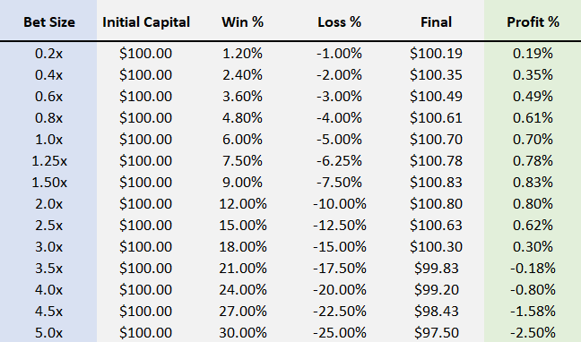
At small bet sizes, the profit grows with leverage in an almost one-to-one relationship. But as leverage increases, the marginal profit shrinks and eventually turns negative. 2x leverage earns less than 1.5x leverage. Greater than 3x leverage actually loses money.

Let’s introduce a new concept, which I will call the Negative Geometric Drag (NGD). This is the “drag” on a portfolio’s profit caused by gaining then losing the same proportion of your net worth.

Remember that's NGD not NdGT.

A gain of X% followed by a loss of X% (or a loss then a gain), will always result in a net loss. For example, if you lose 10% on an investment then make 10% (Investment x 0.90 x 1.10), you are down 1% from your initial investment. Losing 20% and then gaining 20% leaves you down 4% from where you started.

The drag on an investment’s return is the square of the change.

Here’s a table of win/loss bets with no edge (Win % = Loss%). Notice how the Negative Geometric Drag is the square of the bet size (leverage).

Now we can assemble a more complete picture of how leverage affects profit.

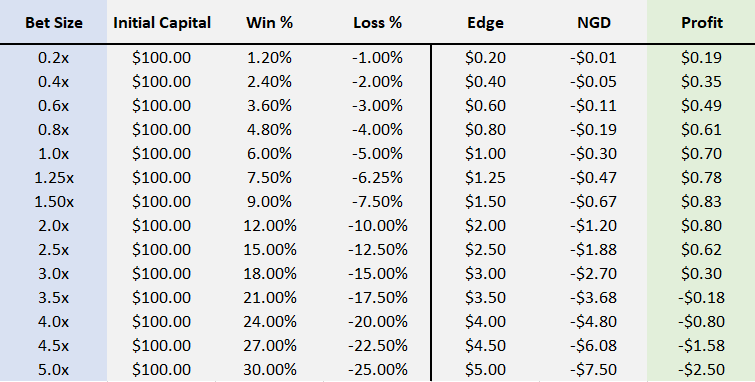
When leverage is increased, the Edge of a bet grows linearly with the amount of leverage but the Negative Geometric Drag (NGD) grows as the square of the leverage.

At lower levels of leverage, the edge is the dominant force and the NGD is negligible. However, as leverage grows, the NGD becomes larger and eventually overwhelms our edge.

Here’s the same 6% vs 5% investment with different levels of leverage. Now the components of Edge, NGD and Profit are broken out individually.

Graphically:

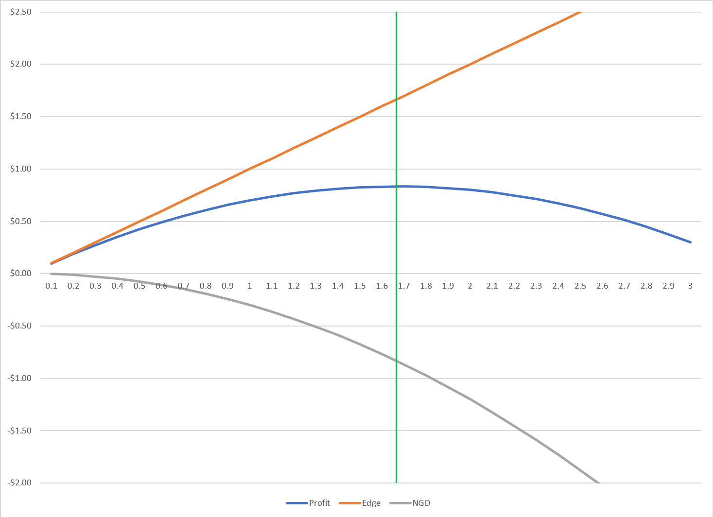
The green vertical line indicates where the two countervailing forces of Edge vs NGD perfectly offset each other (Marginal Edge = Marginal NGD). This is the point of maximum profit (leverage 1.66x), any additional leverage would result in lower profit.

To state this another way, using this level of leverage would maximize the Geometric Growth Rate of your wealth over the course of many bets, investments or trades.

If we ran this experiment over 1,000 bets as we did in the Blackjack example, 1.66x leverage would turn $100 into approximately $6,340. 3x leverage returns only $447 and a reckless leverage of 4x would grind the original $100 down to less than $2.

The Kelly Criterion

Now that we’ve explored the counteracting forces in leverage, we can discuss the Kelly Criterion.

The Kelly Criterion is a formula which accepts known probabilities and payoffs as inputs and outputs the proportion of total wealth to bet in order to achieve the maximum growth rate.

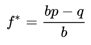
The left-hand side of the equation, f*, is the percentage of our total wealth that we should put at risk. On the right-hand side, p is the probability of a win, q = 1-p is the probability of a loss, and b is the odds (i.e. the ratio of the amount we stand to win to the amount we stand to lose). For example, if we stand to either win $2 or lose $1, we have odds of 2:1 and we would set b to 2.

Applying Kelly to our example investment:

• p = 50%
• q = 50%
• b = 1.2

In this case we have set b = 1.2 to represent the fact that the payout on a win (6%) is 1.2 times the penalty on a loss (-5%). We can then plug these values into the formula:

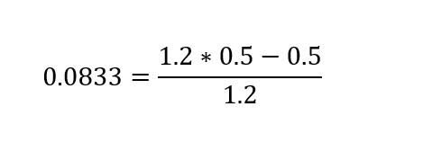
Kelly says to place a bet with a maximum loss of 8.33% of total wealth. Since the base loss in our example is 5%, this implies that we should use a leverage of 8.33% / 5% = 1.66. This is exactly the value that we found earlier.

What about the Blackjack example? The card counter had a 52% chance of winning (p), 48% of losing (q) and even odds (b=1).

The gambler should bet 4% of his bankroll.

Revisiting the graphs and charts above, we can see that Kelly correctly calculated the optimal bet for both scenarios.

From here onward, I’m going present the same familiar Kelly Curve. The Y-axis represents the geometric growth rate, the X-axis represents leverage, and the Kelly-optimal bet lies at the highest point on the curve. In every field of application the general shape of the graph will be the same.

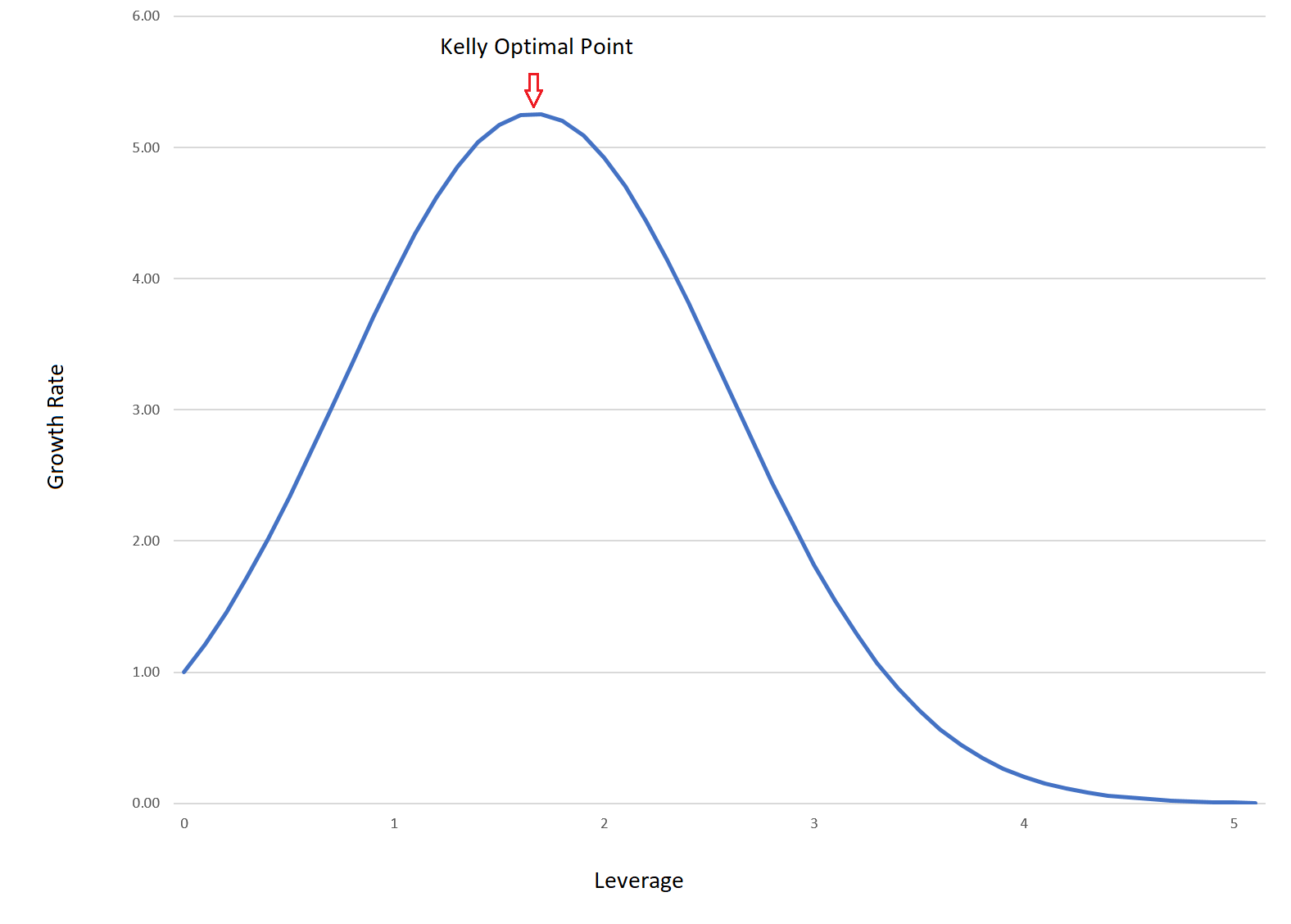
This is a good place to talk about what Kelly Criterion does and what it does not do.

Kelly Criterion DOES:

• Define the point of maximum growth, given known probabilities and known payoffs. (This is rarely applicable to the real world).

Kelly Criterion DOES NOT:

• Calculate the probabilities
• Calculate the payoffs
• Tell us the amount we should actually bet.

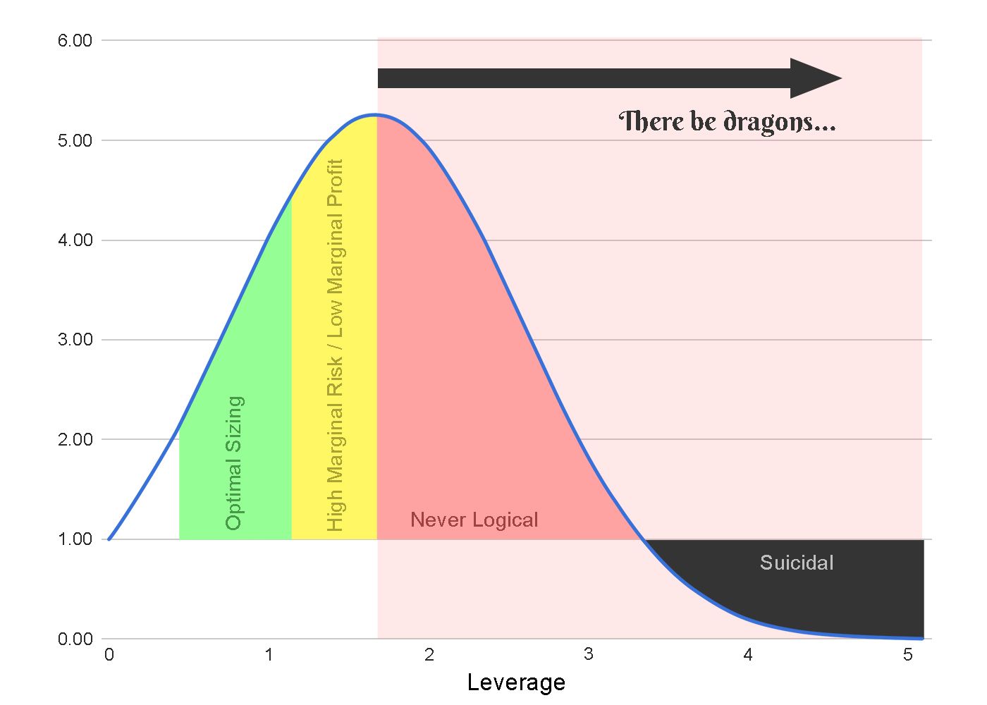
Kelly represents the limit for the range of rational bets. It is the largest bet that could still be rational assuming no value is placed on risk. Betting even one penny more than Kelly would bring increased risk, increased variance and decreased profit.

However, betting anywhere near the Kelly-optimal amount is irrational by most standards.

As the bet size approaches the Kelly-optimal point, the ratio of additional risk to additional profit goes to infinity. Eventually you would have to risk an additional one billion dollars to earn one more cent of expected profit.

Most people assign a negative value to risk. That’s why we pay a premium to insurance companies to haul away excess risk.

For risk-averse actors, the optimal bet is somewhere partway up the Kelly Curve.

Theory vs Reality

“In theory, there is no difference between theory and practice. But in practice, there is.”

To utilize the Kelly Criterion in the real world, I’ll propose two amendments:

1. Be extremely conservative with your assumptions. Take the worst of various possible scenarios. Heavily sandbag your estimates before calculating the Kelly bet.
2. Bet a fraction of the Kelly Criterion (maybe 0.3x or 0.5x).

The first amendment accounts for the fact that the probabilities and payoffs used in the formula are only estimates. The true probabilities and payoffs are hidden, and 9 times out of 10, reality will be less profitable than our estimates.

When investing in an uncertain world, conservative assumptions are closer to reality than expectations. This is known as the “Margin of Safety”.

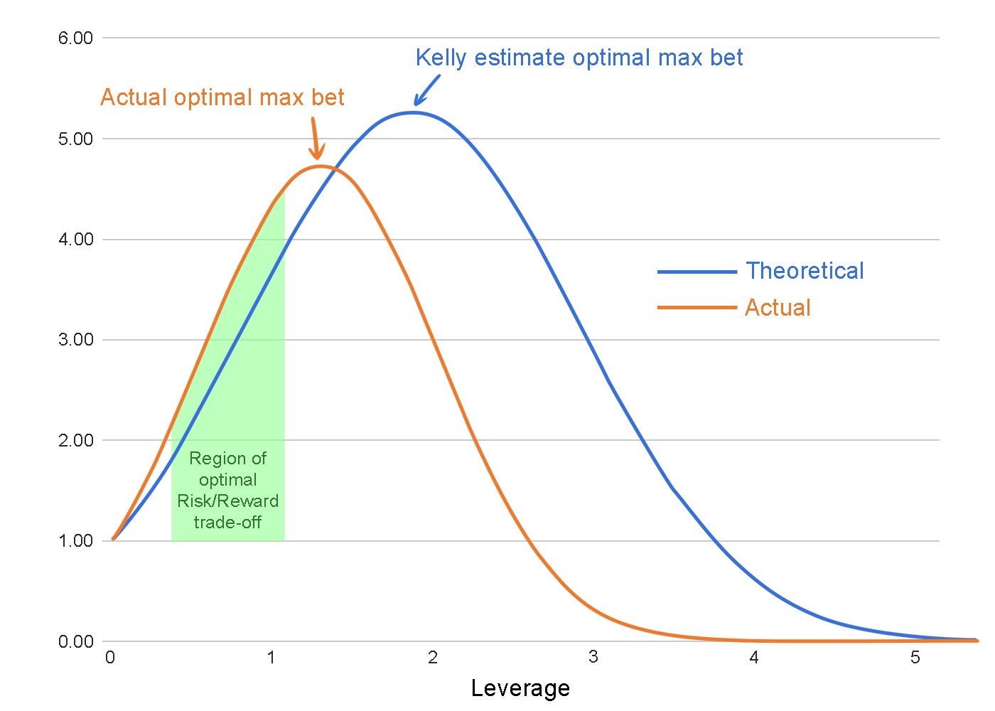
The second amendment results from the observation that a bet sized at 0.3x or 0.5x of Kelly retains a disproportionate amount of the expected profit relative to the variance that it avoids.

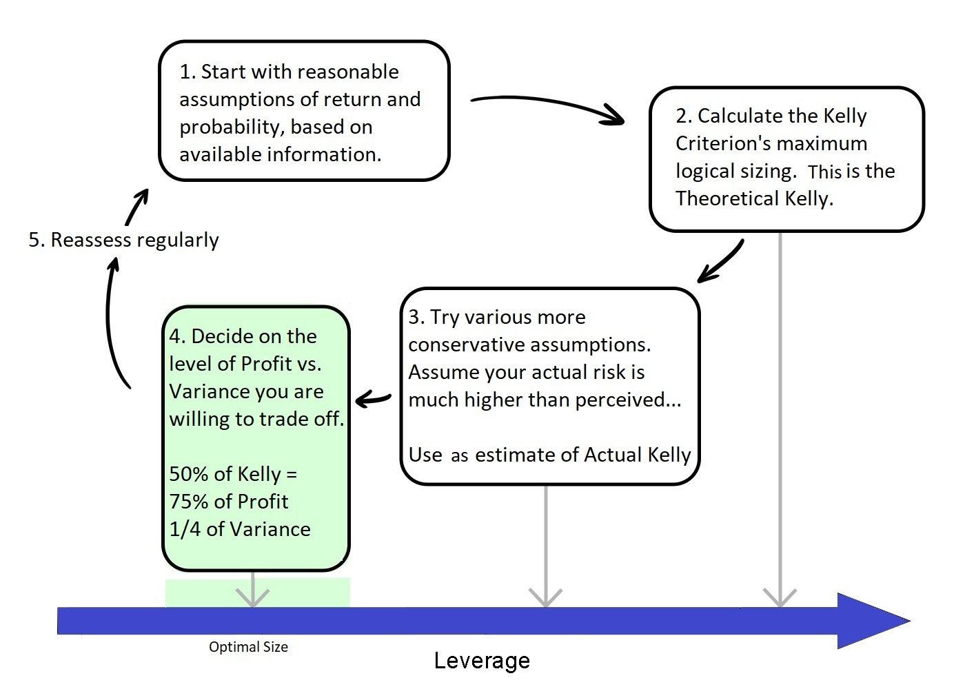
• Betting 50% of Kelly returns 75% of the Kelly-optimal profit with only 1/4th of the variance.
• Betting 30% of Kelly returns 51% of the Kelly-optimal profit with only 1/11th of the variance.

Furthermore, betting fractions of the Kelly-optimal value limits the probability of drawdowns (the amount by which our net worth declines below the highest value achieved so far) by an exponential factor.

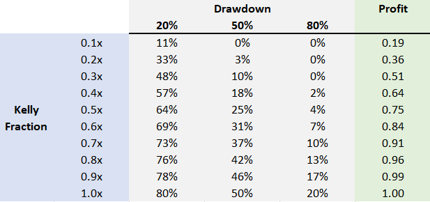
By always betting 30% of the Kelly-optimal bet size, a gambler reduces the chance that he will drop to 20% of his peak bankroll (80% drawdown) from 1-in-5 to 1-in-213, but he still keeps 51% of the growth of a Kelly-optimal bet.

Here is a flow chart for how to approach sizing which incorporates these observations. Remember to constantly reassess all your risks and expectations:

For professional investors - those who manage money for clients - the optimal level of risk is even lower. A drawdown of 30% for a personal investment is fairly common and can be tolerated, but could spell doom for a professional investor with fickle clients.

For money managers, slow and steady is the name of the game. 0.10x-0.15x of the Kelly-optimal investment size is a good rule.

Summary

The Kelly Criterion is a useful tool for assessing the qualitative shape of risk versus reward and understanding boundaries of what is rational. Although it is limited by the exclusion of risk pricing, Kelly can be an excellent tool in the wider arsenal of a quantitative trader. Additionally it provides efficient estimations of drawdowns, variance and geometric growth rate.

“There are old traders, and there are bold traders. There are very few old, bold traders.” -Ed Seykota-

For further reading, here are two excellent books covering the history of markets and the Kelly Criterion:

• Fortune’s Formula by William Poundstone
• A Man for All Markets by Ed Thorp

Don't forget to check out my post on statistical models and betting markets.

Wall Street University: Online Betting Markets

What the 2020 Presidential Election teaches us about Portfolio Theory (and vice versa)

Nick YoderNicholas Yoder